In statistics, an expectation-maximization (EM) algorithm is a method for finding maximum likelihood ormaximum a posteriori (MAP) estimates of parameters in statistical models, where the model depends on unobserved latent variables. EM is an iterative method which alternates between performing an expectation (E) step, which computes the expectation of the log-likelihood evaluated using the current estimate for the latent variables, and a maximization (M) step, which computes parameters maximizing the expected log-likelihood found on the E step. These parameter-estimates are then used to determine the distribution of the latent variables in the next E step.
EM算法可用于很多問題的框架,其中需要估計一組描述概率分布的參數 ,只給定了由此產生的全部數據中能觀察到的一部分!
EM算法是一種迭代算法,它由基本的兩個步驟組成:
E step:估計期望步驟
使用對隱變量的現有估計來計算log極大似然
M step: 最大化期望步驟
計算一個對隱變量更好的估計,使其最大化log似然函數對隱變量Y的期望。用新計算的隱變量參數代替之前的對隱變量的估計,進行下一步的迭代!
觀測數據:觀測到的隨機變量X的IID樣本:

缺失數據:未觀測到的隱含變量(隱變量)Y的值:

完整數據: 包含觀測到的隨機變量X和未觀測到的隨機變量Y的數據,Z=(X,Y)
似然函數:(似然函數的幾種寫法)
D_HBNI489~H%7DGCRMWVJ_thumb.jpg)
log似然函數為:

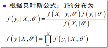
E step:用對隱變量的現有估計 計算隱變量Y的期望

其中需要用到貝葉斯公式:

M step:最大化期望,獲得對隱變量更好的估計

維基中的表述是這樣子:
Given a statistical model consisting of a set  of observed data, a set of unobserved latent data or missing values Y, and a vector of unknown parameters
  , along with a likelihood function
  , the maximum likelihood estimate (MLE) of the unknown parameters is determined by the marginal likelihood of the observed data
)%25ZR_thumb.jpg)
However, this quantity is often intractable.
The EM algorithm seeks to find the MLE of the marginal likelihood by iteratively applying the following two steps:
- Expectation step (E-step): Calculate the expected value of the log likelihood function, with respect to the conditional distribution of Y given
 under the current estimate of the parameters
  :
:
![A7DFNWMY)KAI]T5)_OMKRUD A7DFNWMY)KAI]T5)_OMKRUD](http://www.shnenglu.com/images/cppblog_com/sosi/WindowsLiveWriter/Expectationmaximizationalgorithm_C294/A7DFNWMY)KAI%5DT5)_OMKRUD_thumb.jpg)
- Maximization step (M-step): Find the parameter that maximizes this quantity:

Note that in typical models to which EM is applied:
- The observed data points
 may be discrete (taking one of a fixed number of values, or taking values that must be integers) or continuous (taking a continuous range of real numbers, possibly infinite). There may in fact be a vector of observations associated with each data point.
 - The missing values (aka latent variables) Y are discrete, drawn from a fixed number of values, and there is one latent variable per observed data point.
- The parameters are continuous, and are of two kinds: Parameters that are associated with all data points, and parameters associated with a particular value of a latent variable (i.e. associated with all data points whose corresponding latent variable has a particular value).
However, it is possible to apply EM to other sorts of models.
The motivation is as follows. If we know the value of the parameters  , we can usually find the value of the latent variables Y by maximizing the log-likelihood over all possible values of Y, either simply by iterating over Y or through an algorithm such as the Viterbi algorithm for hidden Markov models. Conversely, if we know the value of the latent variables Y, we can find an estimate of the parameters
  fairly easily, typically by simply grouping the observed data points according to the value of the associated latent variable and averaging the values, or some function of the values, of the points in each group. This suggests an iterative algorithm, in the case where both
  and Y are unknown:
- First, initialize the parameters
 to some random values.
 - Compute the best value for Y given these parameter values.
- Then, use the just-computed values of Y to compute a better estimate for the parameters
 . Parameters associated with a particular value of Y will use only those data points whose associated latent variable has that value.
 - Finally, iterate until convergence.
The algorithm as just described will in fact work, and is commonly called hard EM. The K-means algorithm is an example of this class of algorithms.
However, we can do somewhat better by, rather than making a hard choice for Y given the current parameter values and averaging only over the set of data points associated with a particular value of Y, instead determining the probability of each possible value of Y for each data point, and then using the probabilities associated with a particular value of Y to compute a weighted average over the entire set of data points. The resulting algorithm is commonly called soft EM, and is the type of algorithm normally associated with EM. The counts used to compute these weighted averages are called soft counts (as opposed to the hard counts used in a hard-EM-type algorithm such as K-means). The probabilities computed for Y areposterior probabilities and are what is computed in the E-step. The soft counts used to compute new parameter values are what is computed in the M-step.
總結:
EM is frequently used for data clustering in machine learning and computer vision.
EM會收斂到局部極致,但不能保證收斂到全局最優。
EM對初值比較敏感,通常需要一個好的,快速的初始化過程。
這是我的Machine Learning課程,先總結到這里, 下面的工作是做一個GM_EM的總結,多維高斯密度估計!