老色鬼久久亚洲AV综合,久久r热这里有精品视频,99精品伊人久久久大香线蕉

How to solve AX + XB = C for X using matlab?

杰哥 — Mon, 06 Jul 2015 07:28:00 GMT

X = sylvester(A,B,C)
http://cn.mathworks.com/help/matlab/ref/sylvester.html

杰哥 2015-07-06 15:28 发表评论

Alternating optimization

杰哥 — Sun, 24 May 2015 04:58:00 GMT

Composite Quantization for Approximate Nearest Neighbor Search (ICML 2014)该文�W�三��左侧，倒数�W�五行提到alternative optimization�Q�NeNMF: An Optimal Gradient Method for Nonnegative Matrix Factorization, 该文�W�二��，公式2上面两行�Q�block coordinate descent�Q�以公式2�?��Z��Q�Feature Fusion Using Locally Linear Embedding for Classification提到的参考文献Some Notes on Alternating Optimization;Two-Dimensional Linear Discriminant Analysis的第四页提到的Due to the difficulty of computing the optimal L and R simultaneously, we derive an iterative algorithm in the following.
我个人理解，�q�几个概念都是等��L��?br />

‘alternating optimization’ or ‘alternative optimization’?

Sue (UTS) comment: ‘Alternating’ means you use this optimization with another optimization, one after the other. ‘Alternative’ means you use this optimization instead of any other.

我的GSM-PAF最后用�?/span>‘alternating optimization’

杰哥 2015-05-24 12:58 发表评论

杰哥 — Thu, 05 Dec 2013 11:21:00 GMT

�q�是属于概率��Z��数理�l�计中参��C��计的内容�Q�见教材�W�七章P168�Q�模式识别笔记的Section 3.11.1(Section 3.11到Section 3.11.1的内容应该记�?
�ȝ��Q�最大似然函��C��计法�Q�首先是假设所得的��h��服从某一分布�Q�目标是估计��个分布中的参敎ͼ��Ҏ��是得到这一�l�样本的概率最大时��对应了该模型的参数��|��写出似然函数�Q�再求对敎ͼ�得到�Ҏ��似然�Q�，再求�Ҏ��似然函数的��^均（�Ҏ��q�_��似然�Q�，再对其求��|��得出参数倹{��目前我理解的需要求�Ҏ��的原因是�Q�通常概率是小敎ͼ��q�乘之后会非常小�Q�对计算��言�Q�容易造成��点��C��溢，所以用了取�Ҏ��?br />Zhengxia也提到过似然(likelihood)��是概率�Q�观��到的概率�?br />https://en.wikipedia.org/wiki/Likelihood_function

杰哥 2013-12-05 19:21 发表评论

How to use matlab solve optimization quadratic?

杰哥 — Wed, 21 Nov 2012 10:31:00 GMT

Nannan gives me a fold named "Matlab Help". On page 46 of "Optimization Toolbox User Guide", it lists the constrain and objective type, and the matlab function. For example, if the constrain is linear and the objective is quadratic, we can use quadprog. Note that it can not slove $D_1$ in Section 4.1 of "Smooth minimization of non-smooth functions". Problem: max ((X^T)HX) and H is positive semi definite. The matlab function "quadratic" can not solve this kind of problem. It can only solve the problem: min ((X^T)HX) and H is positive semi definite.

杰哥 2012-11-21 18:31 发表评论

Taylor series in several variables

杰哥 — Wed, 31 Oct 2012 02:48:00 GMT

http://en.wikipedia.org/wiki/Taylor_series

Taylor series in several variables

The Taylor series may also be generalized to functions of more than one variable with

For example, for a function that depends on two variables, x and y, the Taylor series to second order about the point (a, b) is:

where the subscripts denote the respective partial derivatives.

A second-order Taylor series expansion of a scalar-valued function of more than one variable can be written compactly as

where is the gradient of evaluated at and is the Hessian matrix. Applying the multi-index notation the Taylor series for several variables becomes

which is to be understood as a still more abbreviated multi-index version of the first equation of this paragraph, again in full analogy to the single variable case.

[edit]Example

Second-order Taylor series approximation (in gray) of a function around origin.

Compute a second-order Taylor series expansion around point of a function

Firstly, we compute all partial derivatives we need

The Taylor series is

which in this case becomes

Since log(1 + y) is analytic in |y| < 1, we have

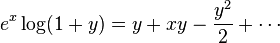
for |y| < 1.

杰哥 2012-10-31 10:48 发表评论

Jensen's inequality

杰哥 — Tue, 30 Oct 2012 04:04:00 GMT

If λ₁ and λ₂ are two arbitrary nonnegative real numbers such that λ₁ + λ₂ = 1 then convexity of implies
[�q�就是凸函数的定义]
This can be easily generalized: if λ₁, λ₂, ..., λ_n are nonnegative real numbers such that λ₁ + ... + λ_n = 1, then

例如-log(x)是凸函数

杰哥 2012-10-30 12:04 发表评论

Gradient Descent(梯度下降�?(两例对应两牛文均用该法求解目标函�?

杰哥 — Fri, 19 Oct 2012 05:33:00 GMT

http://en.wikipedia.org/wiki/Gradient_descent
http://zh.wikipedia.org/wiki/%E6%9C%80%E9%80%9F%E4%B8%8B%E9%99%8D%E6%B3%95
Gradient descent is based on the observation that if the multivariable function is defined and differentiable in a neighborhood of a point , then decreases fastest if one goes from in the direction of the negative gradient of at ,
为啥步长要变化？Tianyi的解释很好：如果步长�q�大�Q�可能��得函数��g��升，故要减小步长 (下面�q�个囄��是在�U怸��d��Q�然后scan�?�?br />Andrew NG的coursera评��Machine learning�?span style="text-align: justify; text-transform: none; background-color: rgb(255,255,255); text-indent: 0px; letter-spacing: normal; display: inline !important; font: 13px/18px Verdana, Helvetica, Arial; white-space: normal; float: none; color: rgb(94,94,94); word-spacing: 0px; -webkit-text-stroke-width: 0px">II. Linear Regression with One Variable�?span style="font-family: 'Calibri','sans-serif'; font-size: 10.5pt; mso-bidi-font-size: 11.0pt; mso-ascii-theme-font: minor-latin; mso-fareast-font-family: 宋体; mso-fareast-theme-font: minor-fareast; mso-hansi-theme-font: minor-latin; mso-bidi-font-family: 'Times New Roman'; mso-bidi-theme-font: minor-bidi; mso-ansi-language: EN-US; mso-fareast-language: ZH-CN; mso-bidi-language: AR-SA" lang="EN-US">Gradient descent Intuition中的解释很好�Q�比如在下图在右侧的点，则梯度是正数�Q?font size="2" face="Arial"> 是负敎ͼ�即��当前的a减小

�?�Q�Toward the Optimization of Normalized Graph Laplacian(TNN 2011)的Fig. 1. Normalized graph Laplacian learning algorithm是很好的梯度下降法的例子.只要看Fig1�Q�其他不必看。Fig1陶Shuning老师课�g 非线性优化第六页�W�四个ppt�Q�对应教材P124�Q�关键直�U�搜索策略，应用非线性优化第四页�W�四个ppt�Q�步长加倍或减倍。只要目标减��就��C��一个搜索点�Q��ƈ且步长加倍；否则停留在原点，��步长减倍�?br />�?�Q?nbsp;Distance Metric Learning for Large Margin Nearest Neighbor Classification(JLMR),目标函数��是公式14�Q�是矩阵M的二�ơ型�Q�展开后就会发玎ͼ�关于M是线性的�Q�故是凸的。对M求导的结果，附录公式18�?9之间的公式中没有M

我自己额外的思考：如果是凸函数�Q�对自变量求偏导�?�Q�然后将自变量求出来不就行了嘛，为啥�q�要梯度下降�Q�上�q�C��二是不行的，因�ؓ对M求导后与M无关了。和tianyi讨论�Q�正因�ؓ求导�? 没有解析解采用梯度下降，有解析解��q��束了

http://blog.csdn.net/yudingjun0611/article/details/8147046

1. 梯度下降�?/strong>

梯度下降法的原理可以参考：斯坦��机器学习第一�?/a>�?/span>

我实验所用的数据�?00个二�l�点�?/span>

如果梯度下降��法不能正常�q�行�Q�考虑使用更小的步�?也就是学习率)�Q�这里需要注意两点：

1�Q�对于��够小�? 能保证在每一步都减小�Q?/span>
2�Q�但是如果太��，梯度下降��法收敛的会很慢�Q?/span>

�ȝ��Q?/span>
1�Q�如果太��，��׃��收敛很慢�Q?/span>
2�Q�如果太大，��׃��能保证每一�ơ�P代都减小�Q�也��׃��能保证收敛；
如何选择-�l�验的方法：
..., 0.001, 0.003, 0.01, 0.03, 0.1, 0.3, 1...
�U?倍于前一个数�?/span>

matlab源码�Q?/span>

[cpp] view plain copy

function [theta0,theta1]=Gradient_descent(X,Y);
theta0=0;
theta1=0;
t0=0;
t1=0;
while(1)
    for i=1:1:100 %100个点
        t0=t0+(theta0+theta1*X(i,1)-Y(i,1))*1;
        t1=t1+(theta0+theta1*X(i,1)-Y(i,1))*X(i,1);
    end
    old_theta0=theta0;
    old_theta1=theta1;
    theta0=theta0-0.000001*t0 %0.000001表示学习�?nbsp;
    theta1=theta1-0.000001*t1
    t0=0;
    t1=0;
    if(sqrt((old_theta0-theta0)^2+(old_theta1-theta1)^2)<0.000001) % �q�里是判断收敛的条�g�Q�当然可以有其他�Ҏ��来做
        break;
    end
end

2. 随机梯度下降�?/strong>

随机梯度下降法适用于样本点数量非常庞大的情况，��法使得��M��向着梯度下降快的方向下降�?/span>

matlab源码�Q?/span>

[cpp] view plain copy

function [theta0,theta1]=Gradient_descent_rand(X,Y);
theta0=0;
theta1=0;
t0=theta0;
t1=theta1;
for i=1:1:100
    t0=theta0-0.01*(theta0+theta1*X(i,1)-Y(i,1))*1
    t1=theta1-0.01*(theta0+theta1*X(i,1)-Y(i,1))*X(i,1)
    theta0=t0
    theta1=t1
end

杰哥 2012-10-19 13:33 发表评论

[zz]Newton Raphson��法

杰哥 — Mon, 15 Oct 2012 23:21:00 GMT
http://blog.csdn.net/flyingworm_eley/article/details/6517853

Newton-Raphson��法在统计中�q�泛应用于求解MLE的参��C��计�?/p>
对应的单变量如下图：

多元函数��法�Q?/p>

Example�Q�（implemented in R�Q?/p>
#定义函数f(x)
f=function(x){
1/x+1/(1-x)
}
#定义f_d1��Z��阶导函数
f_d1=function(x){
-1/x^2+1/(x-1)^2
}
#定义f_d2��Z��阶导函数
f_d2=function(x){
2/x^3-2/(x-1)^3
}

#NR��法　
NR=function(time,init){
X=NULL
D1=NULL #储存Xi一阶导函数�?br />D2=NULL #储存Xi二阶导函数�?br /> count=0
X[1]=init
l=seq(0.02,0.98,0.0002)
plot(l,f(l),pch='.')
points(X[1],f(X[1]),pch=2,col=1)

for (i in 2:time){
D1[i-1]=f_d1(X[i-1])
D2[i-1]=f_d2(X[i-1])
X[i]=X[i-1]-1/(D2[i-1])*(D1[i-1]) #NR��法�q�代�?br /> if (abs(D1[i-1])<0.05)break
points(X[i],f(X[i]),pch=2,col=i)
count=count+1
}
return(list(x=X,Deriviative_1=D,deriviative2=D2,count))
}

o=NR(30,0.9)
�l�果如下图：图中不同颜色的三角�Ş表示i�ơ�P代��生的估计值Xi

o=NR(30,0.9)

#另取函数f(x)
f=function(x){
return(exp(3.5*cos(x))+4*sin(x))
}

f_d1=function(x){
return(-3.5*exp(3.5*cos(x))*sin(x)+4*cos(x))
}

f_d2=function(x){
return(-4*sin(x)+3.5^2*exp(3.5*cos(x))*(sin(x))^2-3.5*exp(3.5*cos(x))*cos(x))
}

得到�l�果如下�Q?/p>
Reference from:
Kevin Quinn
Assistant Professor
Univ Washington

杰哥 2012-10-16 07:21 发表评论

老色鬼久久亚洲AV综合,久久r热这里有精品视频,99精品伊人久久久大香线蕉

How to solve AX + XB = C for X using matlab?

Alternating optimization

How to use matlab solve optimization quadratic?

Taylor series in several variables

Taylor series in several variables

[edit]Example

Jensen's inequality

If λ1 and λ2 are two arbitrary nonnegative real numbers such that λ1 + λ2 = 1 then convexity of implies [�q�就是凸函数的定义]This can be easily generalized: if λ1, λ2, ..., λn are nonnegative real numbers such that λ1 + ... + λn = 1, then例如-log(x)是凸函数

Gradient Descent(梯度下降�?(两例对应两牛文均用该法求解目标函�?

[zz]Newton Raphson���法

[zz]Newton Raphson��法